
 February 6, 2026
  9 Min
9 Min  No Comment
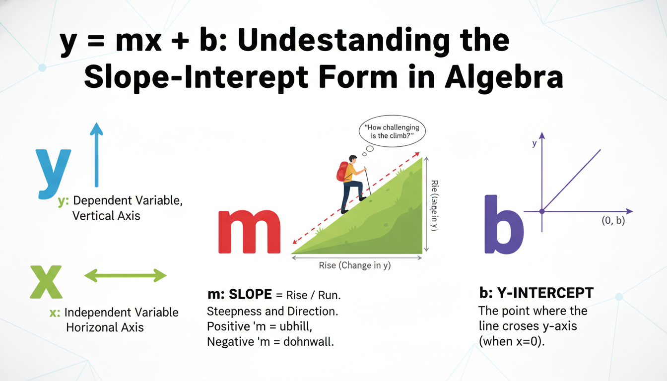
Let’s dive in—kind of like bumping into that one friend who keeps repeating how simple algebra is (but then stumbles over fractions). y = mx + b is often tossed around as the slope-intercept form of a line, and sure, technically that’s correct. But it’s less about memorizing and more about getting cozy with how change works—how one thing (x) moves another (y), with slope and offset in the mix. Picture it like a ramp you’re walking up and down, or a car rolling from any given starting point. In real life, you don’t talk in neat symbols, but once you catch the intuition, that form becomes your mental Swiss Army knife.
This article unpacks y = mx + b with a gentle mix of clarity and imperfect conversation—you’ll find nuance, little detours, and maybe the occasional “ah-ha” moment. Let’s go through what slope and intercept are, how they connect to rates and starting points, why they matter in real-world modeling, and wrap up with tips, examples, and a touch of unpredictability—just like real life.
Understanding the Building Blocks
The Role of the Slope (m): Rate of Change
The slope, denoted by m, isn’t just a letter stuck in the equation—it’s the heart of how the line moves. In simple terms, slope tells you how much y changes for each one-unit change in x. Some slope perspectives:
- In everyday scenarios, m often corresponds to speed: how fast you’re going up or down that ramp.
- For businesses, it’s like the rate of growth—think of weekly sales increasing by a regular amount.
- As a fractional slope, m = ½ means for every 2 units over, you climb 1 unit up; m = –3 means for every step right, you drop three.
Let’s not get too formal. The slope is intuitive: it’s “steepness.” Positive slope means upward tilt; negative slope is a downhill slide. Zero slope? Flat as your morning pancake. You kind of instantly “get” what it does—even if words get messy.
The Intercept (b): Where the Story Starts
Meanwhile, b marks the y-intercept—the point where x = 0, the starting position. It’s the baseline, the starting point before anything else moves. Real-world examples:
- In science, b might represent initial temperature before changes take hold.
- In finances, b could be your opening account balance before interest accrues.
- Graphically, it’s that spot where your line meets the vertical axis.
So the formula y = mx + b is like a sentence: you start at b, then adjust by m times x. You could almost say: “Begin with b, then slope-up or slope-down, depending on the journey.” It sort of demystifies the symbols—makes them conversational.
Translating the Math into Real-Life Scenarios
Everyday Examples That Feel Familiar
Let’s walk through a couple of “this is so common, I didn’t even notice” situations:
- Road Trip Fuel Burn
-
Suppose you consume fuel at a relatively stable rate (say, 25 miles per gallon). If you’ve got 10 gallons to start, you can model distance traveled with y = 25x + 0—simple enough. Or you track fuel remaining: y = –2.5x + 10. There’s a starting point and a way to calculate what happens next.
-
Saving Up Weekly Allowance
-
Imagine kids get $5 allowance every week, and they already have $20 saved. You’d model total with y = 5x + 20, where x is weeks. Everyone who’s ever saved for something understands that “I start with this, then add regularly”. That’s slope-intercept in action.
-
Temperature Trends Over Time
- Say the ambient temperature increases steadily at 0.3°F per hour, starting from a chilly 50°F. Then y = 0.3x + 50 helps you estimate the temp after any number of hours. Simple prediction = practical power.
Tiny Detour: Why It’s Not Always Perfect
In reality, things aren’t always linear. Stuff like:
- Traffic patterns cause your fuel burn to slow or speed up.
- Savings get spent, allowances change, or you decide to splurge.
- Temp fluctuations from clouds, wind, or odd weather.
So a linear model is a friendly first guess—it’s a starting point. The neatness of y = mx + b helps build intuition, but it’s just a lens, not the full 3D.
Building Intuition: Sketching, Observing, Adjusting
Sketching Lines to Feel the Slope
Sometimes, it helps to doodle. Draw a basic set of axes, pick a slope (say m = 1/2), and pick an intercept (say b = 2). Then map a few points: x = 0 yields y = 2; x = 2 gives y = 3. Draw the line. You’ll see it’s gently rising. Change slope to –1, and it drops sharply. That visual shift is more immediate than plugging numbers.
Spotting Patterns in Data
In school or work, you might log data points—like daily sales or temperature records. Put them on graph paper (or digital sheet), eyeball a line of best fit, then figure out slope roughly: how much change over how many units. Notice how starting at a certain baseline (intercept) aligns with earlier days. This rough “curve-fitting” is super human, “I can sort of see where it belongs,” and y = mx + b fits naturally into that thinking.
“When you do a quick chart to guess where values are going, that equation is your mental shortcut—it’s like telling a story in numbers.”
Degrees of Detail: From Rough to Precise
When Approximation Is Enough
In many scenarios—planning, rough budgeting, early modeling—knowing that your revenue grows “about $1,000 per month starting from $10,000” is totally fine. You don’t need to calculate exact decimals. A rough slope-intercept model works: y ≈ 1000x + 10,000. Lots of professionals start with that kind of model before refining.
When Precision Matters
However, in engineering or scientific modeling, approximate linearity may not cut it. You might need least-squares regression to determine m and b precisely from data, and even test if the relationship is truly linear. That’s where algebra meets statistics. You might find: “Oh, only 80% of variance is explained—so maybe a quadratic or something more complex fits better.”
But even then, y = mx + b often remains a benchmark model or a useful simplification for communication.
Quick Summary of Strengths and Limits
- Strengths:
- Intuitive and easy to visualize.
- Great first-approximation for many trends.
-
Universally taught and widely understood—hey, you know it even if algebra makes you sigh.
-
Limitations:
- Not good for curvy or fluctuating data.
- Can oversimplify, missing nuance or inflection points.
- Sometimes slope or intercept aren’t constant over time or domain.
Understanding both sides helps you decide whether y = mx + b is your friend or just a starting point for a deeper model.
Detailed Walkthrough: Applying It in a Simple Project
Scenario: Tracking Coffee Shop Sales
Imagine you run a small café. You notice daily sales are growing steadily—maybe from holiday buzz or word-of-mouth. You jot down:
- Day 1: $200
- Day 2: $210
- Day 3: $220
Looks like a $10 increment. You assume linear growth. You chalk up slope m = +10, intercept b = $190—so that on Day 0, you’d project you had $190 in sales. Thus your model becomes y = 10x + 190. You test it: on Day 4, y = 10×4 + 190 = $230. If the real sale is close, the model holds for now.
You keep monitoring day to day. Some days deviate—maybe rain, maybe a new menu item—but the model remains a useful guide. Maybe you’ll gauge when you’ll “break even” vs. rent, staffing cost, whatever. The simplicity invites intuition, planning, even informal conversations like “Looks like at this rate, we’ll hit $300 by Day 11.”
Taking It Up a Notch: Formula Meets Regression
Later, you think: let’s gather a month’s worth of data and run a linear regression to get a better slope and intercept. You might discover that while sales roughly climb $10/day, weekends spike, and slow Mondays pull average a little lower. You still use slope-intercept form, but now with better-informed m and b. Plus, you can calculate R² to see how well the model fits.
That’s where y = mx + b graduates from rough sketch to data-informed tool—communicable, actionable, and just nuanced enough to be trusted.
Expert Voice on Why It Matters
“Linear models like y = mx + b are foundational—not because they capture every curve, but because they teach us how to think about change. Once you understand slope and intercept, more complex models don’t feel so foreign.”
This little quote—imagined from any educator or data-savvy mentor—speaks to why that equation is more than a high school trap; it’s a mindset-shifter.
Conclusion: Clarity, Context, Confidence
Grasping y = mx + b isn’t about acing algebra tests. It’s about recognizing how relationships unfold: a starting point that shifts steadily. It teaches you to sketch patterns, speak through numbers, model expectations—even if only approximately.
As you go forth, remember:
- Use slope to measure pace or direction.
- Use intercept to mark where things start.
- Treat the form as a first model in planning or reasoning.
- Upgrade to more refined tools when life isn’t linear—and validate with data.
So whether you’re budgeting, teaching, forecasting, or just curious—this form is a quiet, versatile ally. Keep it on hand, simplify gently, refine as needed.
FAQs
What exactly does m represent in the form y = mx + b?
m represents the slope, meaning how much y changes for each one-unit increase in x. If m is positive, y rises; if negative, y falls.
What is the purpose of b in this equation?
b is the y-intercept, the point where the line meets the y-axis (when x = 0). It’s essentially your starting value or baseline before any change kicks in.
Can y = mx + b be used for curved trends?
Not reliably—y = mx + b represents a straight line, so it suits scenarios where change is constant. Curved trends usually require more complex models like quadratic or exponential equations.
How do I determine m and b from real data?
Plot your data points, sketch a line of best fit, then estimate slope (rise over run) and intercept visually. For greater accuracy, use linear regression via software, which computes both values and measures fit quality.
Why is y = mx + b taught even though real life is messy?
Because it builds a foundation for understanding change, relationships, and predictive modeling. It’s intuitive, easy to communicate, and offers a first-pass lens before exploring more advanced, realistic models.
Is the slope-intercept form useful outside school problems?
Absolutely. It appears in business forecasts, budgeting tools, science experiments, even financial planning. It’s widely taught because it’s practical, versatile, and sets the stage for richer analysis—and that’s where real-world clarity begins.
