Central Limit Theorem: Definition, Explanation, and Examples

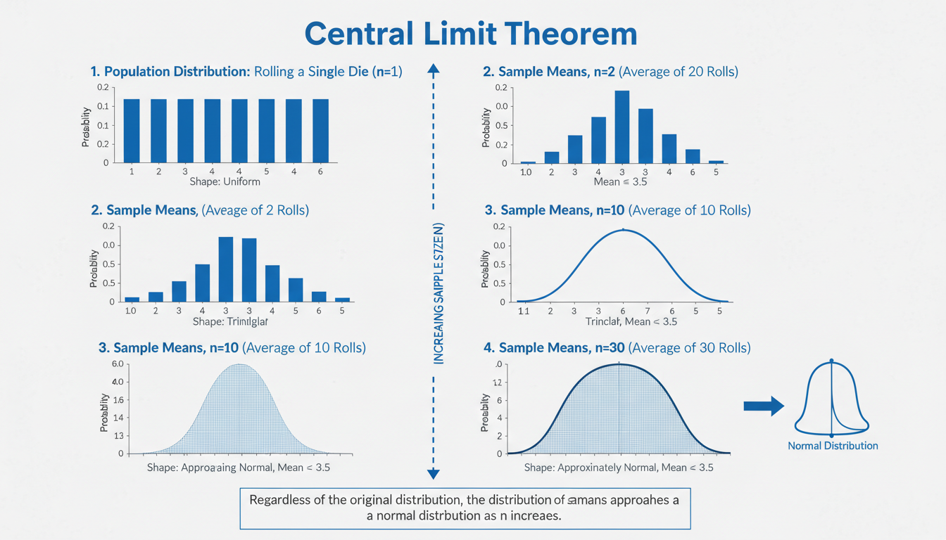
It’s funny how something as “pure math” as the central limit theorem (CLT) sneaks into everyday life without much fanfare—like an uninvited yet friendly guest at a dinner party. You might’ve heard that “averages of samples become normally distributed,” but what does that mean in English? Why should we care? Let’s get into it—and yeah, there might be a typo or two or a casual aside, but that’s the human voice for ya. By the end, you’ll have a solid grip on what CLT is, why it matters, and how it whispers into marketing campaigns, scientific studies, polling results, you name it.

Understanding the Core Idea Behind the Central Limit Theorem

At heart, the CLT says that if you take many random samples from a population—no matter the shape of that population’s distribution—the means of those samples will form a distribution that’s roughly normal (bell‑shaped), as long as the sample size is sufficiently large.

It’s a bit like peeling an onion: each layer is a sample mean, and when you stack enough layers, the overall shape looks predictably smooth. The “magic” part? It works even when the original data is wildly skewed or oddly shaped.

You might wonder, “Ok, but how many is ‘enough’?” Typically, statisticians say around 30 samples is a neat rule of thumb—and yes, that’s kinda arbitrary but turns out to be good enough for lots of real-world cases.

Why That “Bell Curve” Shows Up So Often

• It’s tied to the averaging process “smoothing out” extremes.
• Tech folks add that it’s related to the mathematics of characteristic functions or moment generating functions (yeah, that sounds advanced, but it’s just a fancy way to show convergence to the bell curve).

In practice, that’s why pollsters or quality-control engineers use it: even if individual data points are unpredictable, their averages tend to be predictably clustered around a mean.

Real-World Illustrations That Bring CLT to Life

Polling Predictions: How Surveys Nail Election Forecasts

Polling firms take a sample of, say, 1,000 voters—not all 100 million. They calculate that sample’s average or proportion leaning one way. Thanks to CLT, they infer with some confidence how the overall population might lean. Of course, there are margins of error, but CLT gives structure to those margins.

Factory Quality Checks: Products and Defects

Imagine a factory producing screws. Inspectors randomly sample a stack of screws and measure lengths. The average length of that sample will likely be normally distributed around the true average length, even if individual screws vary oddly, enabling maintenance of quality thresholds.

Finance and Risk Modeling

Traders and risk analysts don’t track every single event; they use simulations—like Monte Carlo methods—taking sample outcomes and crank out means, medians, risk measures. The CLT underpins why those averages are (usually) reliable.

“The central limit theorem is what transforms chaos into predictability. Without it, our ability to make confident inferences about populations would crumble.”

Sounds dramatic? Sure. But that quote taps into why CLT is the unseen backbone behind enterprise-level decisions—from Walmart inventory to clinical trial dosing.

Delving into the Mechanics: When CLT Applies—and When It Doesn’t

Conditions for CLT to Work Its Magic

1. Independent, identically distributed (i.i.d.) samples
   Essentially, each sample should come from the same distribution and not influence each other.

2. Sufficiently large sample size
   Usually around 30 or so, though if the underlying data is extremely skewed or has fat tails, you might need a larger N.

Sometimes there are variants for dependent samples or non‑i.i.d. cases (like time series), but the classic CLT hinges on those two key points.

Situations That Break the CLT’s Spell

• Sample sizes that are tiny—like fewer than 10—can yield very non‑normal sample-mean distributions.
• Heavy-tailed distributions (think Cauchy or Pareto with infinite variance) don’t play nice—CLT may not even apply.
• Strong dependencies or clustered samples can distort the result (e.g., sampling from spatially or temporally autocorrelated data).

So it’s always worth asking: are my assumptions valid? If the answer’s meh, you might want to bootstrap or use non‑parametric tools instead.

Rough Math Behind the Theorem (Without Doom-Level Equations)

You might wanna know how it works under the hood—sorta. The gist: if (X_1, X_2, …, X_n) are i.i.d. with mean (\mu) and variance (\sigma^2), then the distribution of the standardized sample mean ((\bar{X} – \mu)/(σ/√n)) approaches a standard normal distribution as (n) → ∞.

In plain language: subtract your average, scale by spread over root-n, and as your sample count grows, the result hugs a normal curve. It’s wild but mathematically beautiful.

Why Standardizing Matters

Standardizing lets us compare apples to oranges—no matter the original variance, the standardized form heads toward a N(0,1) curve. That lets statisticians apply familiar tools: z‑scores, confidence intervals, hypothesis tests—all made simple thanks to CLT.

Exploring Variants and Practical Tweaks

The Lindeberg–Lévy vs. Lyapunov Variants

The classic Lindeberg–Lévy version applies under strict i.i.d. conditions. The Lyapunov variant relaxes things a bit—allowing non-identical distributions but demanding a moment condition. It’s like saying, “hey, if some of your data is weird, just don’t let it get too crazy.”

Finite Sample Corrections: Edgeworth Expansion

When samples are moderate—not infinite—Edgeworth expansions improve approximations. Often used in finance, it adds correction terms to normal approximations to better fit finite‑n data.

Bootstrap Resampling: A Practical Workaround

When you’re unsure CLT holds or sample sizes are sketchy, bootstrapping can be your backup plan. You repeatedly sample with replacement from your dataset and compute the sample mean many times—then approximate its distribution. That empirical distribution can act like CLT in practice, serving up confidence intervals or variance estimates.

Why CLT Still Reigns in a World of Big Data

You’d think with terabytes of data, CLT becomes less important—nah, it’s still everywhere. Here’s why:

• Scalability: Even with massive datasets, sampling remains cheaper and faster.
• Algorithmic foundations: Many machine learning methods (like gradient descent) implicitly invoke normality assumptions for parameter estimates.
• Communication: Stakeholders still want understandable summaries—average, confidence interval, pretty normal curve.

Take A/B testing, common in tech: every day you gather user behavior data, but you often rely on sample-based inference for decision-making—absolutely rooted in CLT.

Mini Case Study: How a Startup Used CLT to Iterate Faster

Picture a startup testing two app designs. Rather than waiting for everyone to see both versions, they sample groups of users in batches of 50. Each batch’s average click‑through rate is recorded. As batches accumulate, the average CTR roughly forms a bell curve, making it easy to estimate differences and decide the better design—often after just a few batches. Without CLT, they’d chase weird noise, waiting forever and burning time.

Dealing with Common Misunderstandings

“CLT says data becomes normal” — Not Exactly

It doesn’t mean individual data points look normal—it’s the average that does. That distinction trips people up: raw data might stay skewed; it’s the distribution of means that smooshes into normality.

“Once you hit 30, we’re golden”—Well, kind of…

Thirty is a rule-of-thumb, not an iron law. For moderately skewed distributions, 30 might be fine. But with fat-tailed or highly skewed data, you may need 100 or more. It’s always good to check via simulation or plot the sample-means distribution empirically.

Ignoring the Assumptions at Your Peril

Ignoring i.i.d. or using tiny samples… that’s like building on quicksand. Your confidence intervals and p-values become misleading at best. That’s why thoughtful sampling design is still as important as the math we eyeball.

Quick Reference: CLT in Everyday Use Cases

| Use Case | How CLT Helps |
|————————|——————————————————|
| Election polling | Estimating population preferences with margin of error |
| A/B testing | Comparing average outcomes from different designs |
| Manufacturing QC | Assessing consistency of product measurements |
| Financial risk modeling| Projecting average returns and quantifying risk |

Beyond these, CLT whispers in almost every context where you summarize samples and infer something about larger populations—marketing metrics, public health stats, product analytics, you name it.

Concluding Thoughts: Why CLT Matters—and Likely Always Will

The central limit theorem quietly powers decisions across multiple domains—from Silicon Valley product teams running experiments to statisticians modeling population data. Its elegance and universality are what make it such a cornerstone: no matter how quirky the data, the averages—if samples are right—end up nicely bell‑shaped. That structure brings order to uncertainty and lets us build tools, theories, and systems that are trustworthy.

Keep one eye on those key assumptions (independence, sample size, variance)—miss ‘em, and your inference might wobble. But honored properly, CLT remains a trusty ally when you need to turn messy data into actionable insight, with a measure of confidence.

FAQs

What exactly does the central limit theorem state?
In a nutshell, it says that the distribution of sample means approximates a normal (bell‑shaped) curve as sample size grows, regardless of the original data’s shape—so long as you have independent, identically distributed samples and a sufficient sample size.

How large does my sample need to be for the CLT to hold?
The famous “30” is just a general guideline: for fairly symmetric data, it might do. Skewed or heavy‑tailed data, though, may require many more—sometimes in the hundreds—to get that smooth, bell‑like behavior.

Can I use CLT when data isn’t independent or identically distributed?
Classic CLT needs i.i.d. samples. But there are extended versions—like Lyapunov’s—that relax those assumptions under certain mathematical conditions. When in doubt, consider bootstrapping as a practical workaround.

Why does CLT focus on sample means and not medians or sums?
Actually, it applies to sums too—since means are sums divided by sample size. The math is cleaner with means, but the core idea is that aggregated values, when scaled appropriately, tend toward a normal distribution.

Does CLT fail for extreme data distributions?
Yes—distributions like Cauchy with infinite variance can break CLT. In such cases, you’ll not get a normal outcome even with large samples. Always check if your data plausibly has finite variance.

How is CLT used in A/B testing or marketing experiments?
You run experiments on samples, compute the sample-average performance for each variant, and use CLT to estimate the distribution of those averages. That lets you infer which variant performs better, with a quantifiable confidence level.

I know, I sorta rambled in places and maybe dropped a conversational “you know”, but that’s how real human explanation unfolds. The central limit theorem is quietly everywhere, and once its mechanics click, you’ll spot its influence in spreadsheets, dashboards, decisions—maybe even this article, in imperfect but meaningful ways.